
Excel concatenate with delimiter. In this article, you will learn different ways to concatenate strings, cells, arrays, columns, and rows in Excel using the CONCATENATE function and the “&” operator.
In your Excel spreadsheet, the data is not always structured according to your needs. Often you may want to split the contents of a cell into multiple cells, or do the opposite – combine data from two or more columns into a single column. Common examples of having to concatenate in Excel are entering names and addresses, combining text with formula-driven values, displaying dates and times in the desired format, for naming, and so on.
What is “concatenate” in Excel?
In essence, there are two ways to combine data in an Excel spreadsheet:
- Merge cells
- Connect cell values.
When you merge cells, it means merging two or more cells into a single cell. As a result, you have a larger cell displayed across multiple rows and/or columns in the spreadsheet.
When you join cells in Excel, you only concatenate the contents of those cells. In other words, concatenation in Excel is the process of combining two or more values together. This method is often used to combine several pieces of text located in different cells (technically they are called text strings or simply strings ) or insert a value calculated by a formula in the middle of some text.
The following figure shows the difference between these two methods:
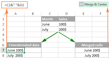
Combining cells in Excel is the topic of our next article, and in this tutorial we will have two workarounds for concatenating strings in Excel – using the CONCATENATE function and the & operator.
CONCATENATE function in Excel
The CONCATENATE function in Excel is designed to join different pieces of text or combine values from several cells into one cell.
The syntax of CONCATENATE is as follows:
CONCATENATE(text1, [text2], …)
Where text is a text string, cell reference, or value in a formula.
Here are a few examples of how to use the CONCATENATE function in Excel.
Connect the values of several cells:
The simplest CONCATENATE formula to combine the values of cells A1 and B1 is as follows:
=CONCATENATE(A1, B1)
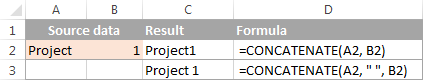
Please note that the values will be knit together without the delimiter, as shown in row 2 in the image below.
To separate values with spaces, enter “” in the second argument, as shown in line 3 in the screenshot below.
=CONCATENATE(A1, ” “, B1)
Concatenate text strings and cell values:
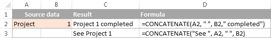
There is nothing that restricts the CONCATENATE function to only concatenate cell values. You can use it to concatenate different text strings to make the results more meaningful. For example:
=CONCATENATE(A1, ” “, B1, ” completed”)
The above formula tells the user that something is done, as shown in row two in the image below. Please note that we add a space before the word ” completed ” to separate the concatenated text strings.
Naturally, you can add a text string at the beginning or in the middle of your Concatenate formula:
=CONCATENATE(“See “, A1, ” “, B1)
A space (“”) is added between the combined values, so that the result shows up as “Project1” rather than “Project1”.
Concatenate a text string and a word value in a calculation formula
To make the result returned by some formula easier to understand for the user, you can concatenate it with a text string to explain what the value actually is.
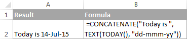
For example, you can use the following formula to return the current date:
=CONCATENATE(“Today is “,TEXT(TODAY(), “dd-mmm-yy”))
Note: Excel concatenate with delimiter
To ensure that your CONCATENATE formulas always yield the correct results, remember these simple rules:
- CONCATENATE requires at least one “text” argument to work.
- In a CONCATENATE formula, you can concatenate up to 255 strings, for a total of 8,192 characters.
- The result of the CONCATENATE function is always a text string, even if all the source values are numbers.
- CONCATENATE is not array-aware. Each cell reference must be listed separately. For example, you should write =CONCATENATE(A1, A2, A3) instead of =CONCATENATE(A1:A3).
- If at least one of the arguments of the CONCATENATE function is not valid, the formula returns the #VALUE! error.
Use “&” to concatenate strings in Excel:
In Microsoft Excel, the & operator is another way to concatenate cells. This method is useful in many cases because typing (&) is much faster than typing “concatenate”.
Similar to the CONCATENATE function, you can use “&” in Excel to combine different text strings, cell values, and results returned by other functions.
Example of “&”.
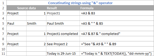
To see the join operator in action, rewrite the CONCATENATE formulas discussed above:
Connect the values in A1 and B1:
=A1&B1
Connect the values in A1 and B1 with the blanks:
=A1&” “&B1
Concatenate values in A1, B1 and a text string: =A1 & B1 & “completed” Concatenate a string and the result of the TEXT / TODAY function: =”Today is ” & TEXT(TODAY(), “dd-mmm-yy”)
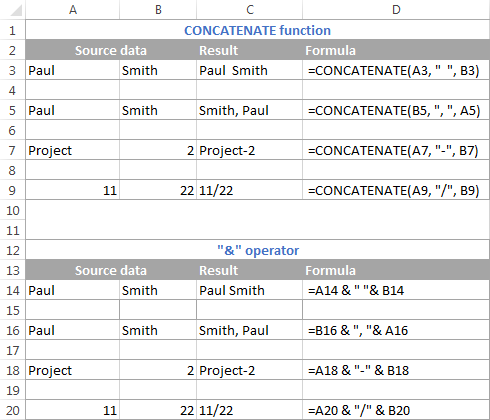
As shown in the screenshot below, the CONCATENATE function and the “&” operator return identical results:
“&” with CONCATENATE function in Excel
Many users wonder if there is a more efficient way to concatenate strings in the CONCATENATE function or the “&” operator.
The only necessary difference between the CONCATENATE and “&” functions is that the CONCATENATE function has a limit of 255 and the & does not. Also, there is no difference between these two concatenation methods, nor is there a difference in validity between the CONCATENATE and “&” formulas.
Since 255 is also a really big number and in practice can never be used up when combining multiple strings, the remaining difference is more comfort and convenience. Some users find the CONCATENATE formula easier to read, personally I prefer to use the “&” method. So just use the splicing technique that you feel more comfortable with.
Connect cells with spaces, commas, and other characters:
In your spreadsheet, you may often have to enter values with commas, spaces, punctuation marks, or other characters such as dashes or slashes. To do this, simply include the character you want to use in your concatenation formula. Remember to enclose that character in quotation marks, as in the following examples.
Connect two cells with a space:
=CONCATENATE(A1, ” “, B1) or =A1 & ” ” & B1
Connect two cells with commas:
=CONCATENATE(A1, “, “, B1) or =A1 & “, ” & B1
Connect two cells with a hyphen:
=CONCATENATE(A1, “-“, B1) or =A1 & “-” & B1
The following figure shows what the result will look like:
Connect text strings with carriage returns
Normally, you would separate concatenated text strings with punctuation marks and spaces, as shown in the previous example. However, in some cases it may be necessary to separate values with a line break. A common example is having to merge mailing addresses from data in separate columns.
One problem is that you cannot simply type a line break in the formula as a normal character and therefore need a CHAR function with the corresponding ASCII code for the concatenation formula:
- On Windows, use CHAR(10) where 10 is the ASCII code for carriage return.
- On Mac systems, use CHAR(13) where 13 is the ASCII code.
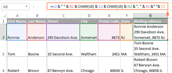
In this example, we have the address parts in columns A through F, and we concatenate them together in column G using the “&” concatenation operator.
Merged values are separated by comma (“,”), space (“”), and carriage return CHAR(10):
=A2 & ” ” & B2 & CHAR(10) & C2 & CHAR(10) & D2 & “, ” & E2 & ” ” & F2
Attention. When using line breaks to separate concatenated values, you must have the option “Wrap text” to allow the results to display correctly. To do this, press Ctrl + 1 to open the Format Cells dialog box , switch to the Alignment tab, and check the Wrap text box.
In the same way, you can separate the concatenated string from other characters like:
Double quotes (“) – CHAR (34)
Cross (/) – CHAR (47)
Asterisk (*) – CHAR (42)
The complete list of ASCII codes can be easily found.
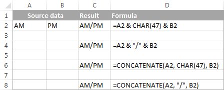
Even so, there is an easier way to insert printable characters in a concatenation formula than simply typing them in quotes like we did in the previous example.
Either way, all four formulas below yield identical results:
=A1 & CHAR(47) & B1
=A1 & “/” & B1
=CONCATENATE(A1, CHAR(47), B1)
=CONCATENATE(A1, “/”, B1)
How to concatenate columns in Excel:
To join two or more columns in Excel, simply enter the normal join formula in the first cell and then copy it down to the other cells by dragging the plus sign (the small square that appears in the lower right corner of the cell). Choose).
For example, to join two columns (columns A and B) separating values with spaces, you enter the following formula in cell C2, and then copy it down to the other cells. When you drag down to copy the formula, the mouse pointer changes to a crosshair, as shown in the figure below:
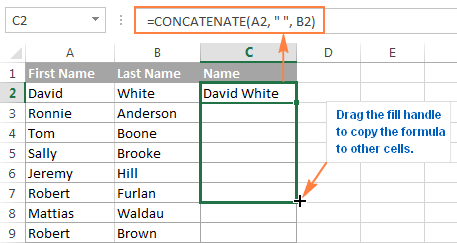
Tips. A quick way to copy a formula down to other cells in a column is to hover over the cell with the formula and double-click the black plus sign
Please note how Microsoft Excel determines where to copy cells after double clicking in the cells with your formulas. If there are blank cells in your table, say cells A6 and B6 are blank in this example, the formula will only be copied to row 5. In this case, you will need to manually scroll down to concatenate. all columns.
How to concatenate an array of cells in Excel:
Combining values from multiple cells can take more work because the CONCATENATE function does not accept arrays and requires a unique cell reference in each argument.
To concatenate several cells, for example A1 through A4, you need one of these two formulas:
=CONCATENATE(A1, A2, A3, A4)
or
=A1 & A2 & A3 & A4
When concatenating a small range, entering all the cell references in the formula is not a big deal. But with many cells, entering each cell manually will be very laborious. Below you will find 3 quick pairing methods in Excel.
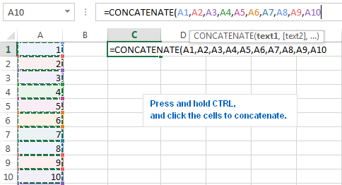
Method 1. Press CTRL to select multiple cells to join
To quickly select several cells, you can press the CTRL key and click each cell that you want to join in the CONCATENATE formula. Here are the detailed steps:
- Select a cell where you want to enter the formula.
- Type =CONCATENATE (in that cell or in the formula bar.
- Press and hold CTRL and click each cell that you want to merge.
- Release the CTRL button, type the closing bracket in the formula bar, and press Enter.
Attention. When using this method you have to click on each cell individually. Selecting a range with the mouse adds an array to the formula, and the CONCATENATE function does not accept it.
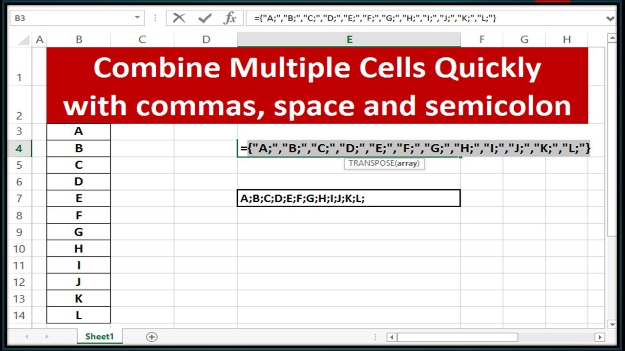
Method 2. Use the TRANSPOSE function to get the range
When you need to concatenate a large range consisting of tens or hundreds of cells, the previous method is not fast enough as it requires clicking on each cell. In this case, a better way is to use the TRANSPOSE function to return an array, and then replace it with individual cell references.
Select the cell that you want to output the concatenated range of.
Enter the TRANSPOSE formula in that cell, for example =TRANSPOSE(A1:A10)
In the formula bar, press F9 to replace the formula with the calculated values.
Removing the curly braces turns a regular Excel formula into an array formula.
As a result, you will have all the cell references to concatenate in your formula.
![]()
Type =CONCATENATE (in front of the cell references in the formula bar, type the closing bracket and press Enter.
Attention. Whichever method you use, the concatenated value in C1 is a text string (notice the data is left-aligned in the cell), even though each value is initially a number. This is because the CONCATENATE function always returns a text string regardless of the source data type.
Concatenate with numbers and dates in different formats:
When you concatenate a text string with a number or date, you may want to format the results differently depending on your data set. To do this, embed the TEXT functions in your Excel formulas.
The TEXT(value, format_text) function takes two arguments:
In the first argument (value), you provide a number or date to be converted to text or a reference to a cell containing a numeric value.
In the second argument (format_text), you enter the desired format of the codes so that the TEXT function can understand.
I will just remind you that when combining a text string and a date , you must use the TEXT function to display the date in the desired format. For example:
=CONCATENATE(“Today is “, TEXT(TODAY(), “mm/dd/yy”))
or
=”Today is ” & TEXT(TODAY(), “mm/dd/yy”)
A few examples of formulas that serialize a text and numeric value are as follows:
=A2 & ” ” & TEXT(B2, “$#,#0.00”) – displays numbers with 2 decimal places and $ sign.
=A2 & ” ” & TEXT(B2, “0.#”) – does not display zeros before commas and $ signs.
=A2 & ” ” & TEXT(B2, “# ?/???”) – displays the number as a fraction.
To be able to apply Excel well in work, we not only master the functions but also have to use Excel’s tools well. Advanced functions help to apply well to work such as SUMIFS, COUNTIFS, SUMPRODUCT, INDEX + MATCH… Commonly used tools are Data validation, Conditional formatting, Pivot table…
Quick video tutorial
Thank you for reading the above tips about the CONCATENATE function in Excel, the application to concatenate strings, cells, arrays and columns. Theartcult hopes this article will be helpful to you!