How to separate text in Excel using formula

How to separate text in Excel using formula. Editing operations on computer applications, especially Excel, are being widely used in daily work, including the learning process. However, you will encounter many difficult situations if you are not familiar with the tools. In order to help you become more proficient in using Excel tools, today let’s learn the quick and effective ways to separate words in Excel right in this article.

Table of Contents:

Why do we need to separate text and numbers in Excel

Reports and spreadsheets may include numbers and text for many reasons. Separating this content serves many purposes and can increase your ability to organize information. Here are some reasons you may separate numbers from text in an Excel document:

Easier to filter: Placing text and numbers in separate columns or rows in Excel allows for easier filtering, sorting and searching. You can use functions and tools to sort columns that contain only numerical data and to filter columns with text.
Increased readability: Having separate columns, rows or cells for text and numbers can make a spreadsheet easier to read and scan. Creating clear, labeled and separated areas for each type of data allows the viewer to identify where to find and place each piece of information efficiently.

How to separate text and numbers in Excel (2 ways)

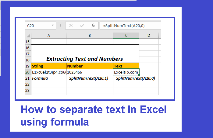
How to separate text in Excel using formula

There are several Excel functions that can be used to split and analyze the text in a data cell as follows:

LEFT function to extract characters from the left side of the text. The syntax of this function is:

= LEFT ( Text, [Number] )

In there:

Text is the text string that you want to extract. Alternatively, it can also be a valid cell reference.
Number is an optional argument that tells the LEFT function how many characters you want to extract from the text string. So this argument must be greater than or equal to 0.

The RIGHT function extracts characters from the right side of the text. This function has the following syntax:

= RIGHT ( Text, [Number] )

In that, the parameters have the same meaning as for the LEFT function described above.

The Find function has the function of finding characters in a text string and the return value is the first position of the first character in the search string. So this function can be used to determine the position of a separator character. The syntax of the function is:

= FIND(SubText, Text, [Start])

In there:

SubText is a string of text that you want to search.
Text is the text string to be searched.
Start is an optional argument that tells the function where to start searching.

The LEN function returns the length of the text string, including the space character. The syntax of the function is:

= LEN ( Text )

Where, Text is the text string that you want to specify the number of characters.

After you understand the function of the functions, let’s combine them together to separate text in Excel. The steps are as follows:

Step 1: We will use the first row (B3) of the sample spreadsheet as an example. First, you combine the LEFT and FIND functions with the following formula:

= LEFT ( B3, FIND( “,”, B3 ) – 1 )

Use the function to separate text in Excel

Formula analysis: In this function, we use the FIND function to get the position of the first delimiter character. The function will return the value 18. Then we continue to use the LEFT function to extract the first element of the text string. Using the ” -1 ” argument makes the LEFT function ignore the delimiter when extracting data. You will then see that the ” Tabbie O’Hallagan ” data has been extracted to cell C3 as a result.

Step 2: In cell D3, you can use the RIGHT function in combination with the LEN and FIND functions with the following formula:

= RIGHT ( B3, LEN ( B3 ) – FIND ( “,”, B3 ) )

Formula parsing: Getting the next elements of a text string is more complicated. You need to remove the first element from the text using the above formula. This formula takes the length of the original text, finds the position of the first delimiter, and then calculates the number of characters remaining in the text string after that delimiter. The RIGHT function then truncates all characters from the right of the text string after the first delimiter. So the result you get will be 056 Dennis Park, Greda, Croatia, 44273 .

Now you can use FIND to locate the next delimiter and the LEFT function to extract the next element with the same steps as above.

How to split text in Excel using the Search function

The Search function will be a useful tool to help you separate text in Excel. The Search function is used to locate a subtext in a total text. You just need to select the place where you want to separate the text in the spreadsheet, then enter the Search function with the syntax:

The syntax to use is:

= SEARCH (find_text,within_text,[start_num])

In there:

find_text : the text, letter, or symbol to find (subtext)
within_text : the total text containing the subtext to find
[start_num] : option where to start searching in within_text

How to split text in Excel using the RIGHT – LEFT – MID . function

In addition, when you want to separate text in Excel , you can use the combination of Right-Left-Mid functions

LEFT . function

The LEFT function separates the exact number of characters from the original text from the left. You just need to select the position to split and then enter the function according to the syntax:

The syntax to use is:

= LEFT (text, [num_chars])

In there:

Text: text
[num_chars]): number of characters you want to get

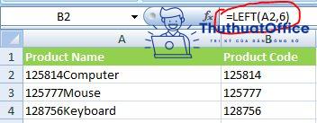
Example: You have a list that includes both codes and names, now you want to separate the product codes into separate columns. You enter the function as follows: =LEFT(A2,6)

In there:

A2: text
6: first 6 characters from left to right

RIGHT . function

The RIGHT function is used to separate text from the right of the original text. You just need to select the position to split and then enter the function according to the syntax:

The syntax to use is:

= RIGHT (text,[num_chars])

In there:

Text: text
[num_chars]: the number of characters you want to split.

The usage and use of the RIGHT function is similar to the LEFT function.

MID . function

The MID function has the effect of getting the value in the middle of the text according to the user’s desire. You just need to select the values you want to split and then enter the function according to the syntax:

The syntax to use is:

= MID (text, start_num, num_chars)

In there

Text: the text you want to get characters
Start_num: the starting point to get the character
Num_chars: number of characters you want to get

Example: You have a product list consisting of company name, product name, and product code. You want to separate the product name. You just need to enter the function: =MID(A1,8,40)

In there:

A1: data cell
8: the starting point of the name.
40: Number of letters in the product.

How to split text in Excel using the LEN . function

The LEN function is not basically a tool to help separate words in Excel, it is often used to count the number of characters in the text. The LEN function itself is also generally only used widely by people who need to be fluent in Excel.

The syntax to use is:

= LEN (text)

For example: You want to count the number of characters of an email in a cell of a spreadsheet just enter:

LEN (” Lillie.Merrit@xyz.com “) = 21. (The LEN function will also count spaces in the text you enter).

The LEN function will have the function of separating letters in Excel when combined with other special Excel word separation functions.

Split text in Excel combines the LEN function and the LEFT . function

Example: You have an email: “ Lillie.Merrit@xyz.com ” and want to separate this person’s name. You use the following:

= LEFT (A2,LEN(A2)-8)

In there:

A2 is the email that needs to be separated
LEN(A2): count the number of characters in mail
-8: subtract the number of characters from the ending “@xyz.com”

Use the Flash Fill tool to separate text in Excel

Flash Fill allows you to include an example of how you want to split your data. Then it will learn and automatically divide the data in the same way as you in other data cells. Therefore, this is considered as a smart tool integrated in Excel.

To split text with the Flash Fill tool, select the first cell that you want to split the data inside and activate the Flash Fill tool (Ctrl + E). Excel will populate the remaining rows based on your example.

In the sample spreadsheet in the article, you will need to enter “Name” in cell C2 and “Tabbie O’Hallagan” in cell C3 . Press Ctrl + E , the data will be split similarly to automatically fill the range from C4:C12 . The rest of the text can do the same.